Wireframe optimization

This tutorial demonstrates several examples of optimizations on wireframes using the Regularized Constrained Least Squares (RCLS) and the Greedy Stellarator Coil Optimization (GSCO) techniques. Further details about these methods may be found in the paper A framework for discrete optimization of stellarator coils.

All examples here make use of the ToroidalWireframe class to formulate the coil current distribution as a set of interconnected straight segments of wire, for which the optimizable parameters are the currents carried by each segment. Each optimization technique upholds the requirement for current continuity; i.e. charge will not accumulate at the nodes where segments intersect.

Regularized Constrained Least Squares (RCLS)

The RCLS technique uses linear least-squares methods to optimize the segment currents with Tikhonov regularization, subject to constraints that include current continuity.

The RCLS objective function to be minimized, subject to the constraints, is defined as follows:

\[J = \frac{1}{2} \int \left| \left(\vec{B}_{wireframe} - \vec{B}_{ext}\right) \cdot \vec{n}\right|^2 ds + \frac{1}{2}\left( \mathbf{W}\vec{x} \right)^2.\]

Here, \(\vec{B}_{wireframe}\) is the magnetic field produced by the wireframe, \(\vec{B}_{ext}\) is the field produced by all other sources including plasma currents and other coils, \(\mathbf{W}\) is a regularization matrix, and \(\vec{x}\) contains the currents in each wireframe segment. The first term in \(J\) is the typical field accuracy objective, while the second term is a Tikhonov regularization objective that penalizes large currents in the segments. Often, the regularization matrix \(\mathbf{W}\) is replaced with a constant factor (in which case all segment currents are penalized by the same factor) or is a diagonal matrix (in which case different segment currents may be penalized by different amounts).

The constraints that may be applied to the wireframe are as follows:

• Continuity constraints. These enforce current continuity at each node of the wireframe where segments intersect. The constraints require the current flowing into each node to equal the current flowing out of it such that charge does not accumulate at the nodes. These constraints are automatically incorporated any time a wireframe is constructed, so there is no need for the user to add them manually.

• Poloidal current constraint. This requires the net poloidal current in the wireframe to have a specified value. Specifying the net poloidal current in this way guarantees a certain average value of the toroidal magnetic field within the wireframe at a certain major radius.

• Toroidal current constraint. This requires the net toroidal current in the wireframe to have a specified value.

• Segment constraints. These constraints require the currents in specified segments to be zero, effectively removing those segments from consideration in the optimization. These are helpful for blocking off sections of the wireframe to reserve space for other components, or for preventing current from flowing across certain user-imposed boundaries.

This section describes two examples of RCLS solutions:

• A basic use case that can be made arbitrarily accurate by increasing the wireframe resolution

• A solution in which segments of the wireframe are blocked off to leave room for ports modeled by Port subclasses

Basic RCLS

The first example includes the fundamental elements of a wireframe optimization using RCLS: creating the wireframe, setting its constraints, setting the optimization parameters, and running the optimization. It can also be found in examples/2_Intermediate/wireframe_rcls_basic.py.

First import the necessary classes, including the ones for creating and optimizing toroidal wireframes:

from simsopt.geo import SurfaceRZFourier, ToroidalWireframe
from simsopt.solve import optimize_wireframe

To construct a ToroidalWireframe class instance, one must specify its geometry and resolution. The geometry is defined according to a toroidal surface, represented by an instance of SurfaceRZFourier, on which the wireframe’s nodes are to be placed. In this example, the toroidal surface is constructed to be a certain uniform distance away from the target plasma boundary.

The nodes are positioned in a two-dimensional grid on the toroidal surface, spaced evenly in the toroidal and poloidal angles. The number of nodes is set by two integers, which specify number of nodes per half-period in the toroidal dimension and the number of nodes in the poloidal dimension, respectively. The geometry of the wireframe segments is fully determined by the node positions, as the segments simply lie on straight lines connecting adjacent pairs of nodes.

The wireframe in the example is constructed as follows:

# Number of wireframe segments per half period in the toroidal dimension
wf_nPhi = 8

# Number of wireframe segments in the poloidal dimension
wf_nTheta = 12

# Distance between the plasma boundary and the wireframe
wf_surf_dist = 0.3

# File for the desired boundary magnetic surface:
TEST_DIR = (Path(__file__).parent / ".." / ".." / "tests" / "test_files").resolve()
filename_equil = TEST_DIR / 'input.LandremanPaul2021_QA'

# Construct the wireframe on a toroidal surface
surf_wf = SurfaceRZFourier.from_vmec_input(filename_equil)
surf_wf.extend_via_projected_normal(wf_surf_dist)
wf = ToroidalWireframe(surf_wf, wf_nPhi, wf_nTheta)

Since the target plasma in this case is a vacuum equilibrium with no internal currents, and the wireframe is the sole magnetic field source, the quantity \(\vec{B}_{ext}\) is zero. Hence, one can trivially optimize the objective function simply by setting all segment currents to zero (\(\vec{x} = 0\)). In order to find a nontrivial solution that produces a nonzero magnetic field with a minimal normal component on the target plasma boundary, it will be necessary to set a constraint requiring the net poloidal current in the wireframe to have a certain value. In the example script, the value is determined by specifying the desired magnetic field near the magnetic axis of the plasma equilibrium:

# Average magnetic field on axis, in Teslas, to be produced by the wireframe.
# This will be used for setting the poloidal current constraint. The radius
# of the magnetic axis will be estimated from the plasma boundary geometry.
field_on_axis = 1.0

# Load the geometry of the target plasma boundary
plas_nPhi = 32
plas_nTheta = 32
surf_plas = SurfaceRZFourier.from_vmec_input(filename_equil,
                nphi=plas_nPhi, ntheta=plas_nTheta, range='half period')

# Calculate the required net poloidal current and set it as a constraint
mu0 = 4.0 * np.pi * 1e-7
pol_cur = -2.0*np.pi*surf_plas.get_rc(0,0)*field_on_axis/mu0
wf.set_poloidal_current(pol_cur)

Finally, the optimization parameters must be specified. For RCLS, this is just the regularization matrix \(\mathbf{W}\):

# Weighting factor for Tikhonov regularization (used instead of a matrix)
regularization_w = 10**-10.

# Set the optimization parameters
opt_params = {'reg_W': regularization_w}

In general, \(\mathbf{W}\) may be an arbitrary matrix. However, for simplicity in this example, a simple scalar value will be used. Effectively, \(\mathbf{W}\) is the scalar times the identity matrix, although it is sufficient to define 'reg_W' as a scalar. Similarly, if one wishes to supply a diagonal matrix for \(\mathbf{W}\), one can simply input the vector of diagonal elements as a one-dimensional array rather than a full matrix.

With all necessary inputs specified, the RCLS procedure may then be run using the optimize_wireframe function. With the wireframe parameters specified above, the optimization itself should take less than a second to perform on a personal computer:

# Run the RCLS optimization
res = optimize_wireframe(wf, 'rcls', opt_params, surf_plas=surf_plas,
                         verbose=False)

When the optimization is complete, the ToroidalWireframe class instance (wf in this case) will be updated such that its currents attribute contains the segment currents found by the optimizer. One can verify that the solution satisfies all constraints using the check_constraints method of the ToroidalWireframe class:

# Verify that the solution satisfies all constraints
assert wf.check_constraints()

In addition to updating the wireframe class instance, the optimize_wireframe function returns a dictionary with some key data associated with the optimization. This includes 'wframe_field', an instance of the WireframeField class representing the magnetic field produced by the optimized wireframe. The WireframeField class is a subclass of the MagneticField class and can therefore be used for subsequent magnetic field calculations.

There are a number of ways to visualize the solution. One way is to generate a two-dimensional plot of the segment currents using the make_plot_2d method of the ToroidalWireframe class:

# Save plots and visualization data to files
wf.make_plot_2d(coordinates='degrees')
pl.savefig(OUT_DIR + 'rcls_wireframe_curr2d.png')

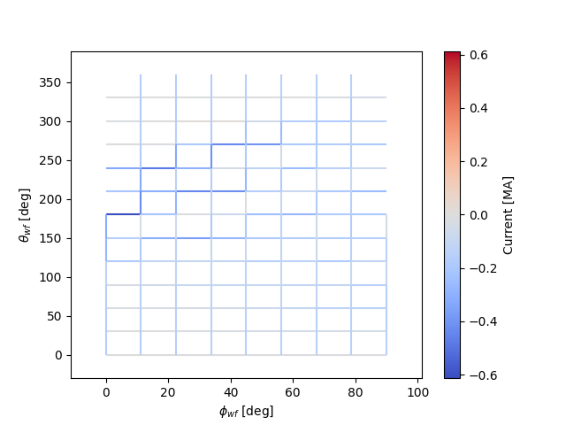
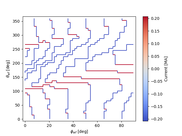
The figure created by this command is shown below. The figure essentially shows the wireframe unwrapped and flattened, with the toroidal dimension running horizontally and the poloidal dimension running vertically. Accordingly, toroidally-oriented wireframe segments are shown as horizontal line segments on the plot, and poloidally-oriented wireframe segments are shown as vertical line segments. By default, a single half-period is plotted; hoever, the user may plot other amounts of the wireframe with the keyword argument 'extent'. The line segments on the plot are color-coded according to the current they carry. Red tones represent positive values, while blue tones represent negative values. For toroidal segments, positive current flows to the right; for poloidal segments, positive current flows upward.

There are also options for generating a three-dimensional rendering of the wireframe. With the to_vtk method, a file will be generated that may be loaded in ParaView:

wf.to_vtk(OUT_DIR + 'rcls_wireframe')

Another option is to use the make_plot_3d method, which generates a three-dimensional rendering using the mayavi package (must be installed separately).

Incorporating ports to avoid

Using the PortSet class, the wireframe can be constrained to have its current distribution avoid overlap with an arbitrary set of ports. The ports may represent actual ports for diagnostics or heating systems, or they could be used more generally to block out spatial regions for other components. This example will modify the above example to ensure that the RCLS optimizer avoids placing currents in segments that overlap a set of ports placed on the outboard side of the stellarator. The ports will be assumed to have circular cross-sections and can thus be represented by the CircularPort class. This example may also be found in the file examples/2_Intermediate/wireframe_rcls_with_ports.py.

First, the general PortSet and CircularPort classes must be imported:

from simsopt.geo import PortSet, CircularPort

The addition of constraints for avoiding ports at certain locations will, in general, reduce the attainable field accuracy at a given wireframe resolution. Thus, the wireframe resolution will be higher than in the previous example in order to achieve a similar level of field accuracy:

# Number of wireframe segments per half period in the toroidal dimension
wf_nPhi = 12

# Number of wireframe segments in the poloidal dimension
wf_nTheta = 22

The location of each port is independently specified by an arbitrary origin point. For convenience in this example, it will be assumed that all ports should have their origins on the same toroidal surface used to generate the wireframe, at specified toroidal and poloidal angles:

# Angular positions in each half-period where ports should be placed
port_phis = [np.pi/8, 3*np.pi/8]  # toroidal angles
port_thetas = [np.pi/4, 7*np.pi/4]  # poloidal angles

Further, for the sake of simplicity, the ports in this example will all have the same dimensions, although in general this need not be the case:

# Dimensions of each port
port_ir = 0.1       # inner radius [m]
port_thick = 0.005  # wall thickness [m]
port_gap = 0.04     # minimum gap between port and wireframe segments [m]
port_l0 = -0.15     # distance from origin to end, negative axis direction [m]
port_l1 = 0.15      # distance from origin to end, positive axis direction [m]

The set of ports (ports) is initialized as an empty instance of the PortSet class:

ports = PortSet()

Each port is then initialized as an instance of the CircularPort class and then added to ports:

# Construct the port geometry
for i in range(len(port_phis)):
    # For simplicity, adjust the angles to the positions of the nearest existing
    # quadrature points in the surf_wf class instance
    phi_nearest = np.argmin(np.abs((0.5/np.pi)*port_phis[i]
                                   - surf_wf.quadpoints_phi))
    for j in range(len(port_thetas)):
        theta_nearest = np.argmin(np.abs((0.5/np.pi)*port_thetas[j] \
                                         - surf_wf.quadpoints_theta))
        ox = surf_wf.gamma()[phi_nearest, theta_nearest, 0]
        oy = surf_wf.gamma()[phi_nearest, theta_nearest, 1]
        oz = surf_wf.gamma()[phi_nearest, theta_nearest, 2]
        ax = surf_wf.normal()[phi_nearest, theta_nearest, 0]
        ay = surf_wf.normal()[phi_nearest, theta_nearest, 1]
        az = surf_wf.normal()[phi_nearest, theta_nearest, 2]
        ports.add_ports([CircularPort(ox=ox, oy=oy, oz=oz, ax=ax, ay=ay, az=az,
            ir=port_ir, thick=port_thick, l0=port_l0, l1=port_l1)])

Remarks about the above code:

• In this example, for simplicity, the port origins (specified by ox, oy, and oz) are not necessarily placed exactly at the toroidal and poloidal angles specified above by port_thetas and port_phis; rather, they are placed at existing quadrature points of surf_wf that are close to the requested angles.

• Each port is set to be locally perpendicular to the surface represented by surf_wf; hence, the port axis (specified by ax, ay, and az) aligns with the local normal vector to the surface represented

Finally, the repeat_via_symmetries method is used to ensure that equivalent ports originating in all half-periods are accounted for:

ports = ports.repeat_via_symmetries(surf_wf.nfp, True)

With the port set fully specified, it can now be used to impart constraints to the wireframe. Note that the PortSet class has a method collides, which takes as input arrays of x, y, and z coordinates of a set of test points and returns a logical array that is True for each point that collides with the port set. This function can be passed as an argument to the constrain_colliding_segments method of a ToroidalWireframe class instance:

# Constrain wireframe segments that collide with the ports
wf.constrain_colliding_segments(ports.collides, gap=port_gap)

Internally, the ToroidalWireframe class instance uses this function to determine which of its segments collide with the port set. Any segments found to be colliding are constrained to carry zero current.

Once these constraints are set, the optimization proceeds in the same way as with the previous example:

# Run the RCLS optimization
res = optimize_wireframe(wf, 'rcls', opt_params, surf_plas=surf_plas,
                         verbose=False)

To generate a 2D plot of the solution, it may be helpful to omit the segments that were constrained to have zero current due to collisions with the ports. This can be done with the quantity keyword parameter to the make_plot_2d method:

# Save plots and visualization data to files
wf.make_plot_2d(quantity='nonzero currents', coordinates='degrees')

While it is possible to output VTK files for the ports and wireframes in order to generate 3D renderings with external software, it is also possible to create 3D images directly in SIMSOPT. For 3D visualizations of wireframes and ports, the mayavi package must be installed. Below is some code that creates a 3D rendering of the plasma boundary, wireframe (with the constrained segments hidden via the keyword argument to_show), and ports:

# Generate a 3D plot if desired
if make_mayavi_plot:

    from mayavi import mlab
    mlab.options.offscreen = True

    mlab.figure(size=(1050,800), bgcolor=(1,1,1))
    wf.make_plot_3d(to_show='active')
    ports.plot()
    surf_plas_plot = SurfaceRZFourier.from_vmec_input(filename_equil,
        nphi=plas_nPhi, ntheta=plas_nTheta, range='full torus')
    surf_plas_plot.plot(engine='mayavi', show=False, close=True,
        wireframe=False, color=(1, 0.75, 1))
    mlab.view(distance=5.5, focalpoint=(0, 0, -0.15))
    mlab.savefig(OUT_DIR + 'rcls_ports_wireframe_plot3d.png')

Greedy Stellarator Coil Optimization (GSCO)

The GSCO technique uses a greedy optimization algorithm that adds loops of current one by one to the wireframe, each time choosing the location and polarization that brings about the greatest reduction of the objective function while upholding certain constraints and eligibility conditions.

The objective function for GSCO is

\[J = \frac{1}{2} \int \left| \left(\vec{B}_{wireframe} - \vec{B}_{ext}\right) \cdot \vec{n}\right|^2 ds + \frac{\lambda_S}{2} N_{active},\]

where \(N_{active}\) is the number of active segments (that is, the number of segments that carry nonzero current) and \(\lambda_S\) is a weighting factor. The first term, which is the same as the first term in the RCLS objective function, incentivizes magnetic field accuracy. The second term incentivizes sparsity in the solution. The higher the value of \(\lambda_S\), the more the optimizer will prioritize sparsity over field accuracy.

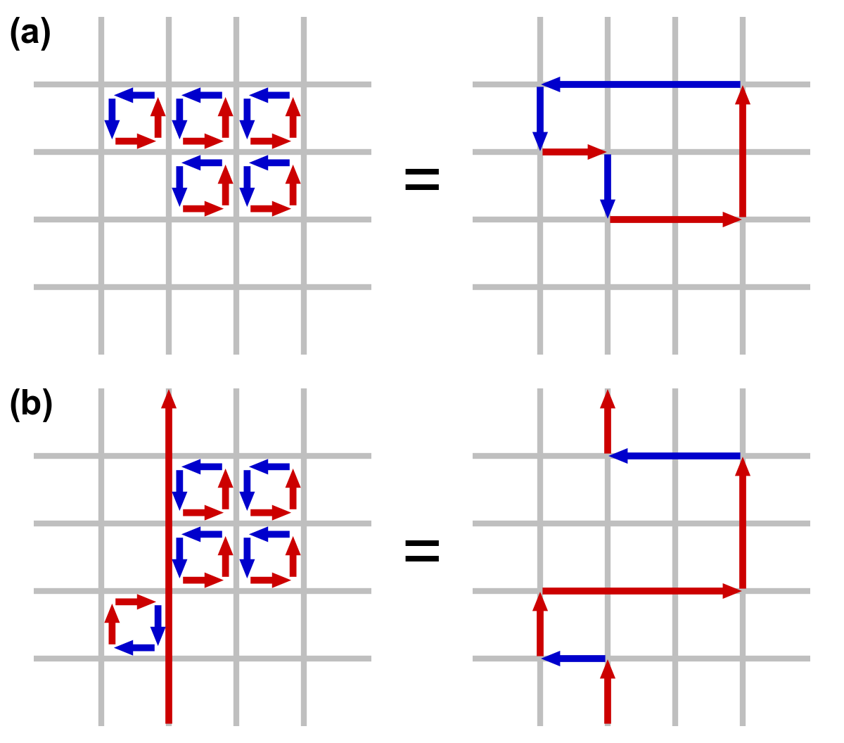
In each GSCO iteration, a loop of current is added to a cell within the wireframe. A cell in this context consists of four segments that form a rectangle in the wireframe grid (i.e. they form a loop that does not enclose any other segments). By adding loops with the same amount of current to adjacent cells in the wireframe, coils can be formed or reshaped. For example, as shown in plot (a) of the figure below, if five loops of current with the same polarity are added to five contiguous cells within the wireframe, the net result will be a single saddle coil enclosing the cells where the loops were added. As another example, as shown in plot (b) of the figure below, adding loops of current to cells adjacent to an initially straight section of a coil will effectively change the shape of the initial coil.

The optimizer cannot necessarily place a loop in any wireframe cell in a given iteration. Whether or not a loop may be added to a given cell is controlled by a eligibility rules. The eligibility rules that may be applied to GSCO optimizations are listed below:

Rule	Description	Parameter in optimize_wireframe
wireframe constraints	Solution must satisfy all constraint equations (this rule is mandatory)	n/a (always applied)
no crossing	At each node, at most two segments may carry current	no_crossing
no new coils	Loops may not be added to a cell around which all segments presently carry no current	no_new_coils
max current \((I_{max})\)	The absolute value of the current in any given segment may not exceed a given \(I_{max}\)	max_current
max loops per cell \((N_{max})\)	The net number of positive or negative loops of current added to a given cell may not exceed a defined maximum, \(N_{max}\)	max_loop_count

The nature of the solution depends greatly on the constraints and eligibility rules that are applied. The examples in this section use the same wireframe structure and optimize for the same plasma, but produce very different solutions by employing different constraints and rules. The examples are as follows:

• Modular coils

• Saddle coils confined to toroidal sectors

• Saddle coils with different currents combined with external toroidal field coils

Modular coils

The first example uses GSCO to produce a modular coil solution. To accomplish this, it is important to note that GSCO cannot create modular coils on an empty wireframe grid, because the current loops added during GSCO iterations can contribute no net poloidal current component. However, if the wireframe is initialized with a set of (planar) TF coils, GSCO can reshape the coils to minimize the objective function. An example of this is demonstrated in the file examples/2_Intermediate/wireframe_gsco_modular.py.

To achieve good field accuracy with GSCO, one generally must use a higher wireframe resolution than what is sufficient with the RCLS approach:

# Number of wireframe segments per half period, toroidal dimension
wf_nPhi = 48

# Number of wireframe segments per half period, poloidal dimension
wf_nTheta = 50

To match the solution in the paper reference, the resolution would need to be increased to 96x100; however, 48x50 already yields a pretty accurate solution.

In this example, the wireframe is created on a surface generated by the BNORM code to be spaced approximately 30 cm from the target plasma boundary. Its coefficients are stored in the format of a NESCOIL input file. This can be used to create a Simsopt surface via the from_nescoil_input method. The surface is then used to create the wireframe:

# Construct the wireframe on a toroidal surface
surf_wf = SurfaceRZFourier.from_nescoil_input(filename_wf_surf, 'current')
wf = ToroidalWireframe(surf_wf, wf_nPhi, wf_nTheta)

Next, a set of planar TF coils is initialized on the wireframe using the add_tfcoil_currents method:

# Calculate the required net poloidal current
mu0 = 4.0 * np.pi * 1e-7
pol_cur = -2.0*np.pi*surf_plas.get_rc(0,0)*field_on_axis/mu0

# Initialize the wireframe with a set of planar TF coils
coil_current = pol_cur/(2*wf.nfp*n_mod_coils_hp)
wf.add_tfcoil_currents(n_mod_coils_hp, coil_current)

The initialized wireframe can be visualized with the make_plot_3d method:

mlab.figure(size=(1050,800), bgcolor=(1,1,1))
wf.make_plot_3d(to_show='all')
surf_plas_plot = SurfaceRZFourier.from_vmec_input(filename_equil,
    nphi=plas_nPhi, ntheta=plas_nTheta, range='full torus')
surf_plas_plot.plot(engine='mayavi', show=False, close=True,
    wireframe=False, color=(1, 0.75, 1))
mlab.view(distance=5.5, focalpoint=(0, 0, -0.15))
mlab.savefig(OUT_DIR + 'gsco_modular_wifeframe_init_plot3d.png')

Before running the GSCO procedure, a number of optimizer parameters must be specified. Among other things, the parameters determine which eligibility rules will be applied for adding current loops to the wireframe. For this example, the “no crossing” rule will be invoked to prevent crossing current paths in the solution by setting the no_crossing parameter to True. It is also necessary to specify the magnitude of the current \(I_{loop}\) in the loops that are added in each iteration. This is done through the default_current parameter. For this application, the best choice is to match the current in the initialized TF coils, as this is the value that is best suited for reshaping those coils without creating forked current paths. Related to this is the maximum allowable current that any segment can carry (max_current). To ensure that no coil in the solution carries more current than the initialized TF coils, this is set to be slightly higher than the default loop current. (It needs to be slightly higher to avoid loops being erroneously marked as ineligible due to floating point imprecision.) The regularization weighting factor \(\lambda_S\) is set through the parameter lambda_S. Finally, a cap on the number of iterations and the frequency with which intermediate results should be saved are set with max_history and print_interval, respectively. To summarize:

# Maximum number of GSCO iterations
max_iter = 2000

# How often to print progress
print_interval = 100

# Weighting factor for the sparsity objective
lambda_S = 10**-6

# Set the optimization parameters
opt_params = {'lambda_S': lambda_S,
              'max_iter': max_iter,
              'print_interval': print_interval,
              'no_crossing': True,
              'default_current': np.abs(coil_current),
              'max_current': 1.1 * np.abs(coil_current)
             }

With the optimization parameters specified, the wireframe can now be optimized:

res = optimize_wireframe(wf, 'gsco', opt_params, surf_plas=surf_plas,
                         verbose=False)

To display the optimized current distributions on dense wireframes with lots of inactive segments, it can improve visual clarity to hide any segments that carry no current. Both the make_plot_2d and make_plot_3d methods offer options for this:

wf.make_plot_2d(coordinates='degrees', quantity='nonzero currents')

wf.make_plot_3d(to_show='active')

Sector-confined saddle coils

While the above example serves as a useful proof-of-concept for the GSCO procedure, it doesn’t take advantage of some of the distinguishing capabilities of GSCO and the wireframe; namely, the ability to control where coils may be placed. In this next example, constraints will be used to produce a design consisting of a combination of planar TF coils and saddle coils that are confined to the sectors in between adjacent TF coils. The example is implemented in the file examples/2_Intermediate/wireframe_gsco_sector_saddle.py.

The setup for this example will be similar to that of the modular coil example, although with a few key differences. First, rather than initializing six planar TF coils per half-period, this example will initialize three to leave more room for the formation of saddle coils in between. Next, to ensure that the GSCO procedure only creates coils between the TF coils and doesn’t reshape the TF coils, constraints will be placed on segments surrounding each TF coil:

# Number of planar TF coils in the solution per half period
n_tf_coils_hp = 3

# Toroidal width, in cells, of the restricted regions (breaks) between sectors
break_width = 2

# Constrain toroidal segments around the TF coils to prevent new coils from
# being placed there (and to prevent the TF coils from being reshaped)
wf.set_toroidal_breaks(n_tf_coils_hp, break_width, allow_pol_current=True)

The constrained segments can be visualized with the make_plot_2d method, setting the quantity argument to 'constrained segments'. Note that the planar TF coils are not visible in this particular plot, but each one runs down through the middle of each of the red stripes:

# Make a plot to show the constrained segments
wf.make_plot_2d(quantity='constrained segments')

Another key difference for this example compared to the modular coil case is in the choice of the loop current \(I_{loop}\) to be used for the GSCO solver. In the modular coil case, the choice of loop current was straightforward: it should match the current of the initialized TF coils such that loops placed next to them could modify their shape without creating forked current paths. However, in this optimization, GSCO will only create saddle coils between the planar TF coils; thus, the TF coil currents are not directly relevant.

Without the need to match the TF coil current, the choice of \(I_{loop}\) is somewhat arbitrary. In general, one should experiment, re-running the optimization with different current levels and seeing which produces the best result. For the example here, setting the loop current to be 5% of the net current used to produce the toroidal field seems to work well. In the paper reference, which uses a higher wireframe grid resolution, a value of 3% is used.

# GSCO loop current as a fraction of net TF coil current
gsco_cur_frac = 0.05

Apart from the constraints and the selection of \(I_{loop}\), the optimization proceeds much the same as for the modular coils, with the same eligibility rules:

# Set the optimization parameters
opt_params = {'lambda_S': lambda_S,
              'max_iter': max_iter,
              'print_interval': print_interval,
              'no_crossing': True,
              'default_current': np.abs(gsco_cur_frac*pol_cur),
              'max_current': 1.1 * np.abs(gsco_cur_frac*pol_cur)
             }

# Run the GSCO optimization
res = optimize_wireframe(wf, 'gsco', opt_params, surf_plas=surf_plas,
                         verbose=False)

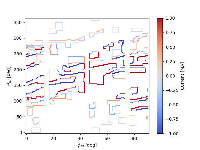
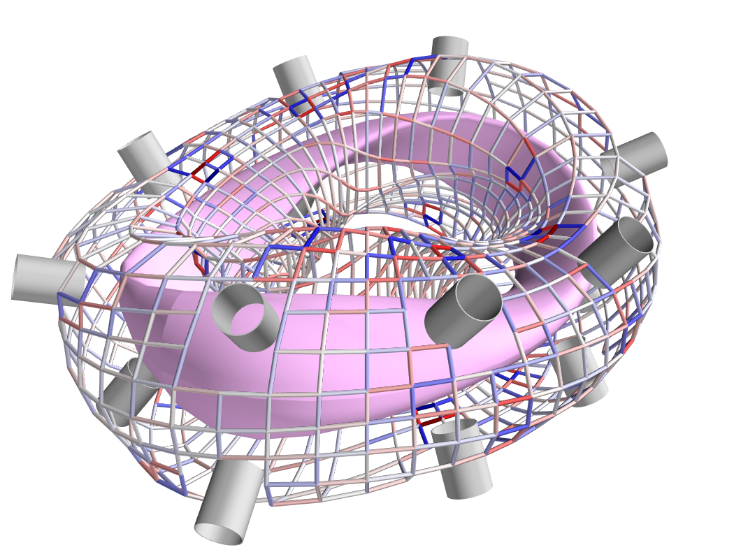
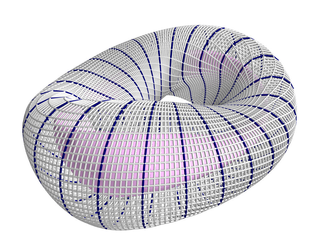
The solution is rendered below in 2D and 3D. The 3D rendering shows a top view with the wireframe solution superimposed on a toroidal surface that takes the shape of the wireframe to emphasize the distinguishing features of this solution. As can be seen in both plots, the TF coils remain planar (vertical in the 2D plot, and forming straight lines radiating from the center of the 3D plot). GSCO has added saddle coils in between each of the planar TF coils. In many cases, the saddle coils are concentric. Note that, as desired, the saddle coils do not touch any of the TF coils and therefore remain confined to toroidal sectors. Such a coil layout is convenient for assembly and disassembly of the device.

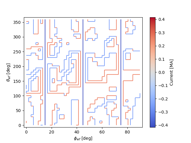
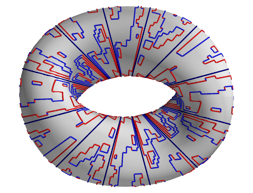
Note that many of the saddle coils form loops that are nested within one another, particularly on the inboard side. This could be (roughly) interpreted as a winding pattern for coils of finite cross-sectional dimensions. In general, using a larger value of \(I_{loop}\) in the optimization will result in less nesting of coils, whereas smaller values of \(I_{loop}\) will result in more nesting. How much nesting can occur is limited by the wireframe resolution (e.g. no nested coils can form inside a coil that is only one cell large), and/or by setting a maximum net number of loops \(N_{max}\) via the “max loops per cell” eligibility rule. The next example avoids nesting using the latter strategy.

Multi-step GSCO optimization

The above two GSCO examples produced solutions in which the non-planar coils were limited to having a single current value. However, it is possible to find solutions with multiple distinct coil currents and other desirable features by applying a sequence of GSCO procedures to a wireframe with carefully chosen constraints. In this example, a solution is found with saddle coils that exhibit multiple current levels and avoid the nesting that was prevalent in the previous saddle coil example. In addition, the toroidal field is supplied by external planar coils rather than from the wireframe itself, illustrating the ability of the wireframe to provide a magnetic field in tandem with other sources.

The basic idea behind this procedure is to perform GSCO multiple times, beginning with a high loop current \(I_{loop}\) and ending with a small \(I_{loop}\). The first step will start from an empty wireframe and add a few saddle coils with the maximum \(I_{loop}\), the second will add on a few coils with a lower \(I_{loop}\), the third will add a few more coils with yet a lower \(I_{loop}\), and so on, resulting in a solution with many saddle soils with several different current values. Empirically, good results have been obtained by halving \(I_{loop}\) for each subsequent step.

A few special measures are taken to avoid potentially undesirable or inconvenient features such as (1) very small coils and (2) nested coils. To avoid very small coils, after each GSCO step the size of each of the new coils is checked. Any coil found to be smaller than a certain size (quantified here by the number of wireframe cells it encloses) is eliminated. Presumably, that small coil produced in step \(n-1\) will be replaced with a larger coil in step \(n\) with a smaller \(I_{loop}\). To avoid the formation of nested coils, two measures are taken. First, the GSCO optimizations apply the “max loops per cell” rule with \(N_{max}=1\). Second, after each GSCO step, any segments that happen to be enclosed within a saddle coil are constrained to carry no current; hence, subsequent GSCO iterations may not place new coils there.

These GSCO steps proceed until the solution converges; i.e. the solution from step \(n\) is no different from the solution from step \(n-1\). At this point, one final GSCO optimization is performed, although the intent in this case is not to add new coils but rather to fine-tune the solution by adjusting the shapes of the existing coils. This can be done by invoking the “no new coils” rule (and/or setting the default \(I_{loop}\) to zero) and running GSCO in “match current” mode. In “match current” mode, during each iteration when GSCO considers the impact on the objective function of adding a loops of current to eligible wireframe cells, for each cell lying next to an existing coil it will adopt as \(I_{loop}\) whatever current happens to be flowing in that adjacent coil. Hence, unlike in the standard mode in which \(I_{loop}\) is restricted to one value, GSCO in “match current” mode can adjust the shapes of multiple coils that have different currents.

To summarize, the multistep procedure in this example goes as follows:

1. Set an initial loop current \(I_{loop}\)

2. Repeat the following until the solution stops changing:

   1. Run GSCO with \(I_{loop}\), invoking the following eligibility rules: “wireframe constraints”, “no crossing”, and “max loops per cell (1)”

   2. Remove any coils that enclose fewer than the minimum number of cells

   3. Constrain segments enclosed by coils to carry no current

   4. Set \(I_{loop} = 0.5 I_{loop}\)

3. Run GSCO in “match current” mode, invoking the following eligibility rules: “wireframe constraints”, “no crossing”, “max loops per cell (1)”, and “no new coils”

This example is implemented in the file examples/3_Advanced/wireframe_gsco_multistep.py. The wireframe is initialized in a very similar way to that of the sector-confined saddle coil example; however with twice the resolution and with no planar TF coils appearing in the wireframe:

# Number of wireframe segments per half period, toroidal dimension
wf_nPhi = 96

# Number of wireframe segments per half period, poloidal dimension
wf_nTheta = 100

# Number of planar TF coils in the solution per half period
n_tf_coils_hp = 3

# Toroidal width, in cells, of the restricted regions (breaks) between sectors
break_width = 4

# Construct the wireframe on a toroidal surface
surf_wf = SurfaceRZFourier.from_nescoil_input(filename_wf_surf, 'current')
wf = ToroidalWireframe(surf_wf, wf_nPhi, wf_nTheta)

# Constrain toroidal segments around the TF coils to prevent new coils from
# being placed there (and to prevent the TF coils from being reshaped)
wf.set_toroidal_breaks(n_tf_coils_hp, break_width, allow_pol_current=True)

The toroidal field will be provided in this case by an external set of circular, planar coils:

# Number of planar TF coils in the solution per half period
n_tf_coils_hp = 3

# Create an external set of TF coils
tf_curves = create_equally_spaced_curves(n_tf_coils_hp, surf_plas.nfp, True,
                                         R0=1.0, R1=0.85)
tf_curr = [Current(-pol_cur/(2*n_tf_coils_hp*surf_plas.nfp))
           for i in range(n_tf_coils_hp)]
tf_coils = coils_via_symmetries(tf_curves, tf_curr, surf_plas.nfp, True)
mf_tf = BiotSavart(tf_coils)

The initial value of \(I_{loop}\), to be used in the first GSCO step, is chosen to be 20% of the net poloidal current used to generate the toroidal field:

# GSCO loop current as a fraction of net TF coil current
init_gsco_cur_frac = 0.2

The series of GSCO optimizations is performed within one while loop. Prior to starting the loop, a number of updating variables must be initialized:

# Initialize loop variables
soln_prev = np.full(wf.currents.shape, np.nan)
soln_current = np.array(wf.currents)
cur_frac = init_gsco_cur_frac
loop_count = None
final_step = False
encl_segs = []
n_step = 0

soln_current and soln_prev hold, respectively, the current solution and the solution from the previous step. They are used to determine whether the solution has changed from one step to the next. cur_frac effectively determines what \(I_{loop}\) should be for each GSCO procedure and is initialized here prior to the beginning of the while loop. loop_count is an array with one element per wireframe cell that keeps track of how many loops have been added to each cell during a GSCO procedure (it is updated by the GSCO function). Nominally, loop_count must have the same number of elements as wireframe cells, but if it is set to None, the GSCO function will interpret this as an empty grid. However, in subsequent steps, loop_count will be an array containing the data on loops added in previous steps, and subsequent calls to GSCO will add to this loop.

Steps 2-3 of the summarized procedure above are implemented in a single while loop since much of the code for steps 2a-d and step 3 is the same. Whether or not an iteration of the while loop is in step 2a-d or step 3 is determined by the logical variable final_step. In turn, final_step is initialized as False and set to True only once the solution stops changing (soln_prev == soln_current). Note that the initialization of soln_prev and soln_current above will prevent the first iteration of the while loop from being the final step:

# Multi-step optimization loop
while not final_step:

    n_step += 1

    if not final_step and np.all(soln_prev == soln_current):
        final_step = True
        wf.set_segments_free(encl_segs)

One of the distinguishing features of steps 2a-d and step 3 are the optimization parameters used by GSCO, as shown below. Steps 2a-d use a nonzero default current. By contrast, step 3 (active when final_step == True) invokes the no_new_coils rule, operates in match_current mode, and uses a default_current of zero. Note that, in step 3, it is necessary to set the max_current to (slightly above) the initial current to allow GSCO to adjust the shape of coils carrying the initial (highest) current level:

# Set the optimization parameters
if not final_step:
    opt_params = {'lambda_S': lambda_S,
                  'max_iter': max_iter,
                  'print_interval': print_interval,
                  'no_crossing': True,
                  'max_loop_count': 1,
                  'loop_count_init': loop_count,
                  'default_current': np.abs(cur_frac*pol_cur),
                  'max_current': 1.1 * np.abs(cur_frac*pol_cur)
                 }
else:
    opt_params = {'lambda_S': lambda_S,
                  'max_iter': max_iter,
                  'print_interval': print_interval,
                  'no_crossing': True,
                  'max_loop_count': 1,
                  'loop_count_init': loop_count,
                  'match_current': True,
                  'no_new_coils': True,
                  'default_current': 0,
                  'max_current': 1.1 * np.abs(init_gsco_cur_frac*pol_cur)
                 }

Conveniently, with opt_params set suitably for the respective stage of the procedure, the call to optimize_wireframe() is the same. Note that, unlike in the other examples in this tutorial, an external field (ext_field) must be provided corresponding to the field provided by the external TF coils:

# Run the GSCO optimization
res = optimize_wireframe(wf, 'gsco', opt_params, surf_plas=surf_plas,
                         ext_field=mf_tf, verbose=False)

If final_step == False, the above call to optimize_wireframe() constitutes step 2a of the above procedure. Before moving on to the next GSCO stage, steps 2b-c must be conducted. First, any saddle coil smaller than the user-designated minimum size is removed from the solution. The coil sizes are obtained with the helper function find_coil_sizes included in the file. The removal of the coils is implemented through a modification of the currents array of the ToroidalWireframe class instance. Specifically, any segment that had been a part of the small coils has its current set to zero. Additionally, the loop_count array, which is not contained within the ToroidalWireframe, must be updated. Then, within all the new saddle coils (at least those that weren’t removed for being too small), the wireframe segments are constrained to carry zero current:

if not final_step:

    # "Sweep" the solution to remove coils that are too small
    coil_sizes = find_coil_sizes(res['loop_count'], wf.get_cell_neighbors())
    small_inds = np.where(\
        np.logical_and(coil_sizes > 0, coil_sizes < min_coil_size))[0]
    adjoining_segs = wf.get_cell_key()[small_inds,:]
    segs_to_zero = np.unique(adjoining_segs.reshape((-1)))

    # Modify the solution by removing the small coils
    loop_count = res['loop_count']
    wf.currents[segs_to_zero] = 0
    loop_count[small_inds] = 0

    # Prevent coils from being placed inside existing coils in subsequent
    # steps
    encl_segs = constrain_enclosed_segments(wf, loop_count)

Assuming this is not the last step, i.e. final_step == False, the last steps before the next while loop iteration include halving \(I_{loop}\) (as per step 2d of the above procedure) and updating soln_prev and soln_current:

cur_frac *= 0.5

soln_prev = soln_current
soln_current = np.array(wf.currents)

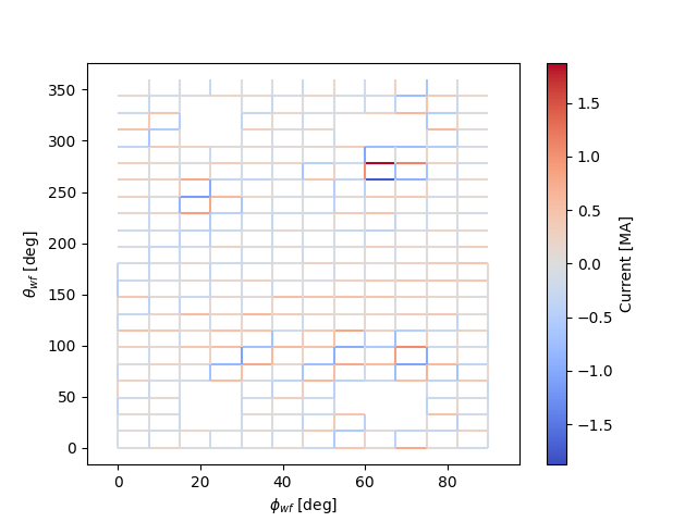
The end result of this multistep procedure is shown in 2D and 3D below.